May 01, 2016

This is a (very, very, very¹ delayed) response to an article on slider interfaes published last year by Baymard Institute. The article goes beyond what will be considered here — and you should read it.

Sliders are often used to give a visual cue in content filtering; the user drags a slider to a position corresponding to some value, and content is then filtered according to that value.

Linear slider scales provide a poor user experience, because the underlying data is rarely a uniform distribution. This creates two problems; large portions of the slider may represent no change in the filtering, and small portions may represent huge changes in the filtering. The article suggests solving these problems with the use of biased, logarithmic, or exponential scales. Real-world data often fits nicely on either a logarithmic or exponential curve, but not always. I propose the use of histogram equalization for creating biased scales — a custom mapping from slider-positions to values in the underlying data. In fact, I expect this solution to fit any dataset you might come up with.

Lenshawk lenses by focal length

Before I go further in-depth with the solution, let’s see an example. The two sliders below simulate filtering on the freely available Lens Hawk dataset, referenced in the Baymard article. For simplicity, instead of showing all the lenses that match the filter, the number of matches is displayed.

According to the article, Lens hawk uses an exponential scale for filtering on focal length. You can try it out here.
(Note: Their scale is 4-800, mine is 45-8000.)

Linear slider

Biased slider

We can immediately see that, at the middle of the slider, the linear scale matches 548/561 lenses (98%), where the biased scale matches 269/561 lenses (48%).

This means the right half of the linear-scale slider is used for only 2% of the items, while the remaining 98% is crammed into the left half. If you play with the sliders a little, you will notice that the linear scale puts nearly all of the lenses within the first ∼12% of the slider, while the biased scale distributes the lenses quite evenly.

So does the biased scale above provide a better user experience? While it seems like a vast improvement on the linear scale, it shifts the focus. On the linear scale, it is difficult to control the number of matching items, but on the biased scale, it is difficult to control the exact filter value!

If the relationship between the number of matched items and the filter value can be made apparent, the biased scale is a huge improvement. When you know of this relationship, it is easy to see that, for a less-than-or-equal filter, the highest value lower than the wanted max matches the exact same items as the wanted max value. But my guess is most people would find the biased scale unintuitive, and be annoyed that they can’t pick the exact value they want. Of course, this is just conjecture.

This is where the logarithmic or exponential scales win; their smoothness seems to make them easier to use and understand, despite the non-linearity. Probably, a solution that weighs smoothness against scale utilization is possible.

Histogram Equalization

A common problem in image processing is contrast adjustment. Contrast adjustment is used for example by photographers, for aesthetic purposes, and scientist have found use for it in image segmentation, which is important used for things like computer vision and medical image analysis (If you’ve ever had an MRI, CT, or X-ray, the resulting images have likely been histogram-equalized).

Histogram equalization works for many types of data, but the canonical example is monochrome images. Pixels in a monochrome image can have values between the two extremes; black and white. But just like we didn’t have lenses with every possible focal length between 4.5 and 8000 in the Lenshawk example, you can have images that don’t utilize the space between black and white very well. It might be that there are no or few values in the brighter end of the spectrum (much like our Lenshawk example), or it might be that there are mostly very dark and bright values, but not much in between. Histogram equalization is used to assign new values to the image pixels, to better utilize the spectrum.

There is a direct correspondence between the problem of contrast adjustment, and our problem of slider scaling. In contrast adjustment, we want to maximize the use of the colour-range. In slider scaling, we want to maximize the use of our slider range. Same thing, kind of.

There is an important difference between the two problems. In contrast adjustment we may change the actual colours in the image, but in slider scaling we may not adjust the values of the items we are filtering. As it turns out, this is not a big problem — we don’t want to change the underlying values, just how our slider maps to them!

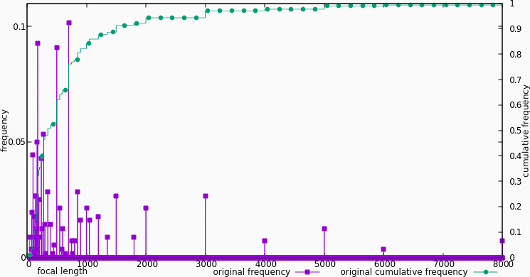
Distribution of lenses over focal-length

In order understand how histogram equalization can help (and what it is), let’s take a closer look at the problem. The figure above shows the frequency and cumulative frequency of different focal lengths, normalized to 1. As you can see, most of the lenses, by far, lie in the [0, 1000] range, while the [6000, 8000] range is almost empty! Ideally, we want the cumulative frequency to be a line. That would mean the data was uniformly distributed, and thus all equal-sized segments on the slider would cover the same number of items. In the Lenshawk dataset, the cumulative frequency looks like a log curve, not a line.

The histogram equalization algorithm works as follows:

1. Go through the data, for each unique value, store the number of times that value occurs, divided by the size of the data set. This gives us the frequency histogram above. We can see this as a function from focal-length to the percentage of lenses with that focal length.

2. Go trough the histogram, in order of increasing value, and store for each value the sum of the frequencies for all values smaller than or equal to the value. This gives us the cumulative frequency function as above. We can see this as a function from focal length to the percentage of lenses with that or a smaller focal length.

3. Scale and translate the cumulative frequencies from the [0, 1] range, to the wanted range. For contrast adjustment, it would generally be the range of possible color values in the image format. In our case, it’s the range of slider inputs, [0, 8000]. We can see this as a function from focal length, to a focal length in an imagined data set, that is more evenly distributed.

Normally, you would create a new data set by applying the resulting mapping to each value in the original data. For slider scaling however, we simply pretend that our slider is the new data set, and then use the inverse of the mapping to get the value represented by a point on the slider!

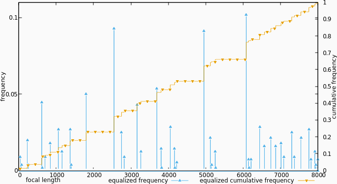
Equalized distribution of lenses over focal-length

If we pretend that we did build a new data set, and then calculate the frequency histogram and cumulative frequency of it, we get the figure above. The frequencies are he exact same as before, but are distributed differently over the focal lengths (which are really slider positions now). The cumulative frequency is a lot more linear than originally.

Footnotes